What I learned building a small text-to-image model
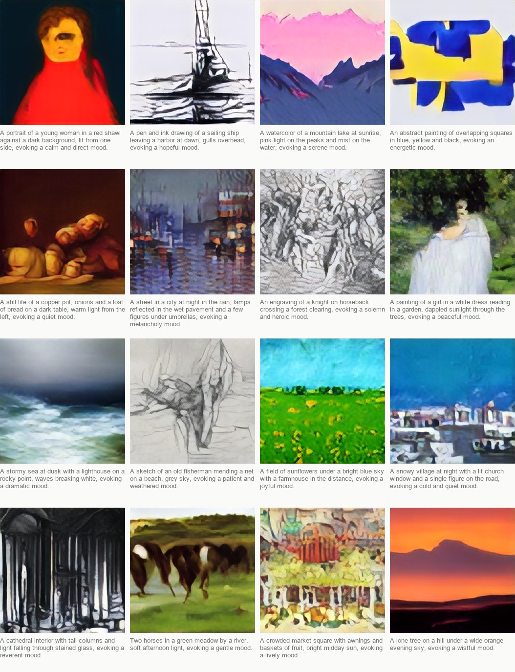
A sample of 16 images generated from sentences describing a variety of different subjects, styles, and moods.
Overview
This article follows a project called lit2img, which renders sequences of images from input text. I worked on this purely for fun. I've recently been looking for projects I could complete that would bring me a sense of joy, which is something I long for in my work these days. Enjoyable software-related work, for me, often contains elements of storytelling and information visualization. One previous project that comes to mind was Limbus, a very basic tool for visualizing the running sentiment of text over time. I built Limbus with the idea that it would be fun to visualize linguistic signals (like emotional sentiment) over the course of a novel.
This time around, I was interested in learning more about text-to-image models. I set out to experiment with building a tool for generating frames of images from sequences of text. The specific goal was to learn more about how these models work by building, training, and evaluating one from scratch, and to enjoy experimenting with the model as it produced visual output. I explicitly did not intend to build a model that was "useful" for any purpose other than this exploration.
In general, I lament the use of text-to-image models for things like advertising and publishing. Even so, I find it fascinating to learn about how these models work.
One of the most compelling uses of LLMs in my own experience, outside of professional work, is in their use as guides through new topics of study. Throughout this project, I engaged Claude models (Fable 5.1 and Opus 5.5) to build a learning path through the design of each stage of the project. In an initial prompt, I explained the overarching goal, including my own learning objective, the constraints, and a requirement to iteratively build upon an index of concepts in the domain. This prompt generated a high-level sequence of modules, each of which covered a specific aspect of the architecture or training and serving processes.
Over the course of about a month, I spent several evenings a week writing and generating code for each module and reading papers about concepts as they were introduced, based on examples provided by the LLM. I found it useful to treat the code output of the frontier model like traditional print material, and the prose surrounding the code as a conversation with the author about the topic or implementation. As the LLM generated code implementing each part of the model in its output, I chose to transpose most of it manually, as I would if I were using a book. This preserved a kind of slowness that I feel is important in learning.
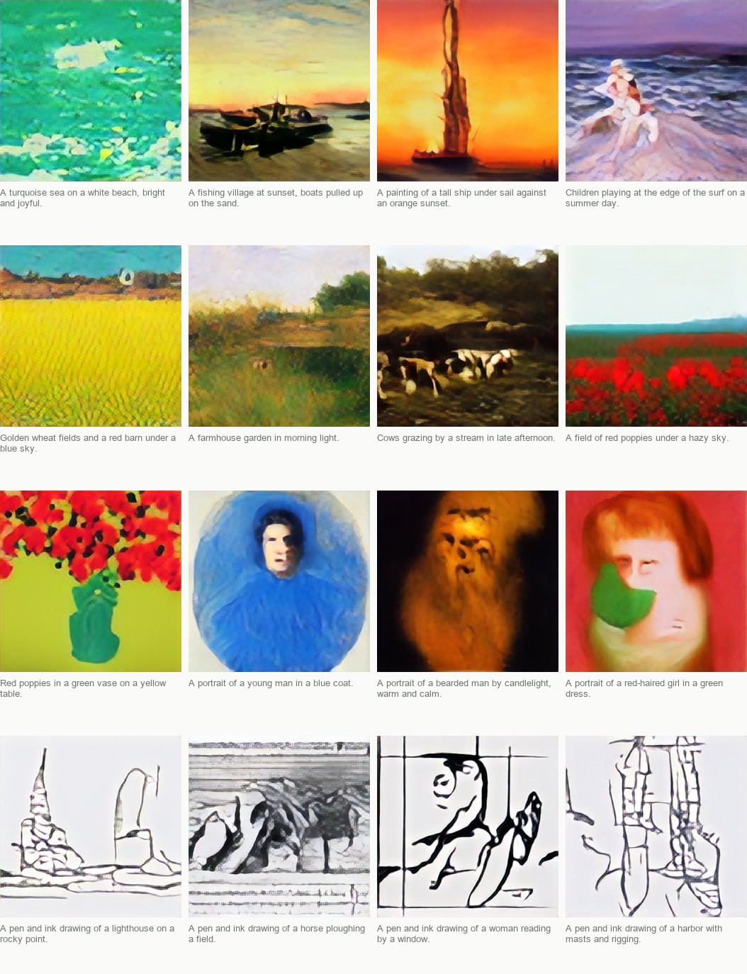
Sixteen more generated images, with the sentence that produced each one printed under it.
General Learnings and Takeaways
On the AI/ML side of things, I suspect the issues I encountered are obvious to folks who do this work professionally. However, a few takeaways from the project seem to generalize well beyond the purely technical learnings. This was the first significant personal project in which I used a frontier model to act primarily as a "guide" through topics that were new to me.
- Using frontier models for learning a new subject, or deepening my understanding of an existing topic, can be valuable. However, I'm still left with the feeling that I don't know what I don't know. I knew nothing about the mechanics of latent diffusion (Stable Diffusion), CLIP, diffusion transformers (DiT), or Classifier-Free Guidance prior to starting this project. From that perspective, it was a great experience working with the LLM to build a structured learning path through the relevant technology while building. As I worked, I produced a running HTML artifact that provided definitions of useful terms and ideas. This preserved a kind of dynamic study guide that I could read while not producing code, which I feel improved my understanding over time. However, with previous experience only on the text side of the model, I wonder how long it would have taken me to piece together the necessary knowledge to construct and sufficiently understand the ideas behind this model without such an easily-manufactured guide. Are there important technical mistakes or oversights that I made along the way? I still don't know, because I relied on my own interaction with a frontier model to serve as a guide for my learning. It's possible that more exploratory prompting could've helped uncover more unknowns. It still seems that using LLMs as learning companions unlocks a massive potential for self-learners. However, I'm not sure that it entirely replaces reading curated research, controlled experimentation, and, in particular, human mentorship. These traditional avenues for learning are much slower processes, and typically have the explicit objective of learning rather than producing. The LLM-as-mentor approach seems to occupy a much murkier area, a hybrid of learning and the rapid production of a completed result. Even when that completed result is learning "material," it's now far too easy to slip out of self-directed learning and into "build mode." I'm curious to learn how other folks use frontier models as learning companions. I'm a believer in "building to learn," but, without care, this path feels more like "watch it get built to learn," which is an illusory form of learning, especially as a beginner. I don't become a much better pole vaulter by watching an Olympic athlete compete; I need some adequate combination of watching and doing to develop skillfully.
- I feel a kind of attenuation in my capacity to sit with a problem. I've often felt my capacity to learn is a well-developed tolerance for "being stuck for long periods of time with a lack of understanding." From now on, there is always a trade-off; ask the LLM and get un-stuck, as it pertains to your next output objective, or stay stuck for longer periods of time in relative ignorance in order to exercise your capacity to learn. I believe deep human learning will continue to require direct effort in training one's capacity to sit with not-knowing, and often in taking the winding path that emerges when solving problems "manually." There is immeasurable value in walking these winding paths to experience acts of learning. I should write more about that sometime.
- On the ML side of things, there is generally a loss floor. It took me a while to understand why the loss could reach some asymptotic value while the images produced by the model continued to get "better." A large part of the loss is irreducible. At high noise levels, the original image can't be recovered from the input, so the best any model can do is predict a kind of "average." While a loss that moves from 1.136 to 1.127 looks small, if the floor is near 1.100, the part the model can actually improve has dropped by a quarter! Reading the loss as if zero were the goal is not a reasonable expectation. The loss number always has some constant offset. One way to look at this is to find out, for any given measurement (in ML or anywhere else), how good it can possibly be. Once information has been lost, no change in the model can recover it.
With those takeaways in mind, what follows is a summary of the project itself.
Breaking the project down into two problems
Building a text-to-image model involves working on "text input" and "image generation" as two fairly distinct problems. The first is encoding text as something a network can use -- a vector, or a sequence of vectors, that carries meaning. The second is generating images, given some input text.
Each sub-problem is interesting on its own. So, I split the project into two parts, along these lines. I kept a small number of important constraints throughout development. First, I wanted to start small enough to train on my laptop (a MacBook Pro with PyTorch's Metal backend), and second, I wanted to write the constituent parts by hand, and stop to ask questions along the way to improve my understanding. As a result, I built the original tokenizer, attention, residual blocks, autoencoder, samplers, and the evaluation metrics using only PyTorch's primitives.
I'd like to clarify what parts of this model I built "by hand." While I built and trained a tokenizer and transformer for the text side of the model myself, in the end, as I will describe, I replaced it with a pre-trained text encoder, trained on a much larger and broader dataset. The parts of the model that generate images, the autoencoder and the diffusion model, I wrote and trained myself. I also wrote the samplers and the code that evaluates the results. In the final model and training pipeline, all parts that read text or judge images use pre-trained models. The text encoder in the final model is a pre-trained one from OpenAI, the captions were written by a pre-trained vision model, and the metrics I report lean on pre-trained models.
Text Side
The text side of the model starts with a tokenizer. For this, I implemented a fairly standard byte-level byte-pair
encoding tokenizer. This approach, used by models like
GPT-2 and
RoBERTa, tokenizes text as byte sequences, rather than as characters. UTF-8 writes any character as one
to four bytes, and a byte has 256 possible values. The tokenizer starts from those 256 and grows its vocabulary by repeatedly merging the
pair of adjacent tokens that occurs most often in the corpus. The character “é” is the two bytes C3 A9; an untrained tokenizer uses two
tokens to represent it. If it is common in the corpus, the merge of C3 A9 eventually occurs, forming a single token. A rare character,
like a Chinese character in an English corpus, remains unmerged as three or four bytes. Using this approach, rather than an a priori
character-based tokenizer with a fixed alphabet, nothing is ever unrepresentable. The cost of rarity is additional tokens rather than
information. A pre-tokenization pass splits the text into words (with their leading spaces), digits, and punctuation first, which ensures
that merges never straddle two words; this is a convenient heuristic, given that most English words are separated by a space, and
sentences end with punctuation.
Three characters from a byte-level BPE tokenizer perspective. A common letter is one byte and one token. "é" is two bytes. A BPE may merge these into a single token by seeing it frequently relative to all other byte-pairs in a corpus. A rare character is three bytes that likely never merge into a single token.
BPE training learns an ordered list of merges; encoding applies that list to new text in the same order. Here "Call me Ishmael" goes from fifteen bytes to ten tokens over the course of five merges.
I trained the tokenizer on twenty public-domain novels and used GPT-2's tokenizer as a benchmark, comparing my token count to GPT-2's for the same text. I did this on Moby Dick (seen in training) and on Pride and Prejudice (which I held out from training).
| vocab | Moby Dick tokens | ratio vs GPT-2 | held-out ratio |
|---|---|---|---|
| 512 | 599,565 | 1.833 | 1.860 |
| 2,048 | 413,058 | 1.263 | 1.269 |
| 8,192 | 332,737 | 1.017 | 1.042 |
At 8,192 entries, a vocabulary about six times smaller than GPT-2's encodes Moby Dick within 2% of GPT-2's token count, and the held-out ratio is only 0.5-2.5% worse than the seen one, so the merges seem to generalize reasonably well. The texts in the public domain were likely narrow enough in terms of text information variance that it's unsurprising that a tokenizer with a much smaller vocabulary produced similar token count to GPT-2's tokenizer, which was trained to efficiently tokenize a massively broader corpus of text.
I built a 5.25M-parameter decoder-only transformer, also in the GPT-2 family, with causal self-attention and rotary position embeddings. Position encoding turns out to be a surprisingly deep topic. The systems I worked on around 2015 used word2vec and had no concept of position at all, and the history from sinusoidal encodings to rotary is fascinating to me. I'd like to write about it in a separate post some day.
One head of causal self-attention, the key mechanism of the transformer. Each token is projected to a query, a key and a value. Scores above the diagonal are masked before the softmax; a token can only attend to itself and the tokens before it, it learns nothing from any token that comes after it, chronologically.
After a minimal amount of local training, prompting the transformer model with “Call me Ishmael,” generated somewhat comprehensible prose. It was interesting to see invented words emerge, like "unrecained" and "punoken," both phonetically plausible, as the training progressed. As I increased the amount of text during training, the invented words gradually stopped appearing. It's interesting to see, throughout the project as a whole, that the outputs from relatively small models improved dramatically by adding more data.
Image Side
This is the part of the project I learned the most from, as I'd never worked with diffusion models prior to this exploration. Diffusion training adds noise to an image and trains a network to remove it. Given a noisy image, a diffusion model can predict the noise that was added (ε), the clean image (x₀), or a particular mixture of the two (v). These are algebraically interchangeable; given any one of them, you can compute the other two. What differs in each case is the loss. Because the quantities have different scales at different noise levels, choosing a target implicitly chooses how much each noise level contributes to the gradient. Measured as error on the clean image, predicting ε puts most of the weight on the low-noise steps, predicting x₀ weights every noise level equally, and v sits between the two.
There is a fourth option, called flow matching. Flow matching does away with the noise schedule and
draws a straight line from image to noise, xₜ = (1−t)·x₀ + t·ε. Along a straight line, the velocity is constant, so the network learns one
vector field and generating an image is solving an ODE backwards.
This is one of the more complex ideas in the model, and I plan to write a follow up article exploring and visualizing flow matching in more detail.
I trained all four approaches on 32-pixel images and scored them with FID, which embeds real and generated images with a frozen classifier and measures the distance between the two distributions, lower being better.
| target | final val loss | best FID |
|---|---|---|
| ε | 0.061 | 35.0 |
| flow matching | -- | 36.8 |
| v | 0.114 | 40.9 |
| x₀ | 0.049 | 51.8 |
As you can see, validation loss and FID do not track each other. The x₀ model has the best loss and the worst FID; the ε model has a middling loss and the best FID. The training objective (in this case, the FID) and the loss did not produce the same ranking. I suspect this overarching problem of "scoring" different approaches is another complex topic worth exploring in more detail; something I imagine engineers in the ML and AI space must wrestle with as part of real-world problem solving.
In any case, flow matching with 50 network evaluations came within two FID points of ε with a thousand. Therefore, I chose to continue with flow matching as the prediction target.
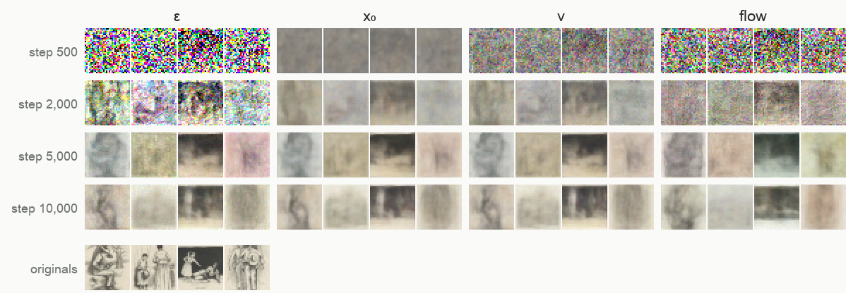
The same architecture trained with four different prediction targets. Each cell is the model's estimate of the clean image from the same heavily noised inputs, at four points in training; the originals are shown in the bottom row.
Looking at the data
The training images come from two sources: 81.4k paintings from WikiArt, and 1k illustration plates from Project Gutenberg's HTML editions. It seemed intuitive that captioned images from text would provide reasonable text-image pairs. Unfortunately, I discovered that captions rarely exist in the markup. Here, I decided it would be interesting to generate the captions using a pre-trained local model. I produced the captions with Qwen2.5-VL 7B, quantized to 4 bits and running locally at about 60 tokens per second. The model was prompted for one sentence per image, set up to name what is shown, the setting, and the mood. The 1,075 plates took about forty minutes to complete. Looking at the images, it also became clear that many weren't illustrations in the sense I was looking for, but page scans with small drawings, etc. After a validation split was held out and the page scans were dropped, 78,308 images were left for training.
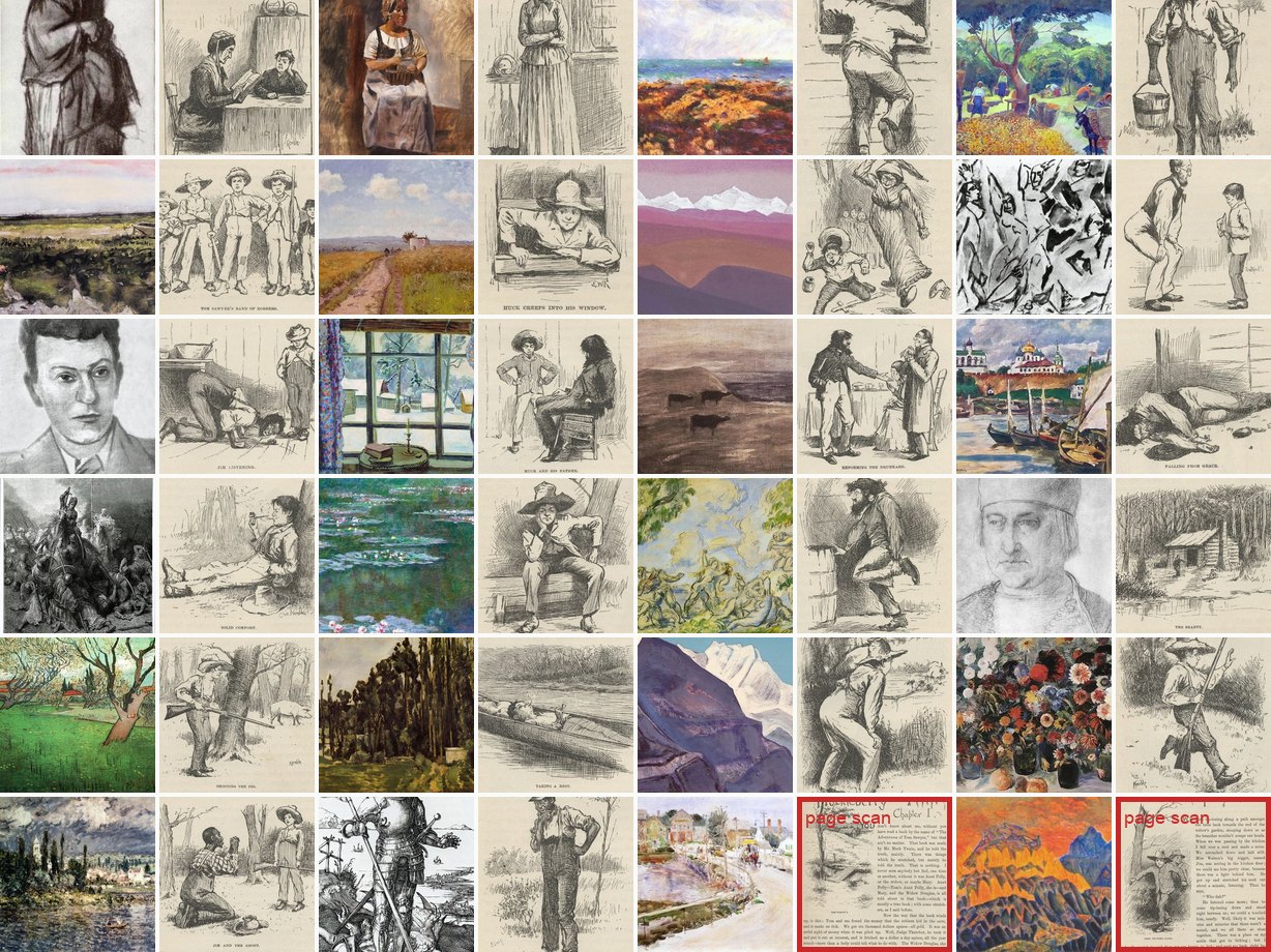
Looking at the data found several problems, including page scans that were not illustrations, and printed captions baked into images.
There are many interesting considerations related to training image selection and captioning, and I wish I could spend more time here exploring how increasing the size and variance of the training data and captioning methods would generalize the model output. I feel that so much of the end result of this project is the result of the selection of the training image dataset and the captions that label them. My thought here is that since this model learns to produce images using patterns strictly from the training image dataset, which is a small and narrow space, the space of possible outputs that encode visual meaning is limited and highly curated. Similarly, I suspect that there is very low variance in the structure and content of the language used to caption the images, based on my approach to use a single model to auto-label each image with the same prompt. I'm thinking that this highly constrained space of training data likely enables the model to produce interesting results within a narrow band of image style and subject matter, and likely produces loosely structured noise outside of that space.
The ceiling
Up to this point I had been working with 32-pixel images. Moving to 256×256 pixels meant that the network had to handle 196,608 numbers per image. Furthermore, it had to do that at each of the many steps of sampling, which quickly became impractical. The approach I learned about, which comes from the Stable Diffusion paper by Rombach et al., is to first compress each image into a much smaller representation, called a latent, and to run diffusion on the latents rather than on the pixels.
For this, I built a convolutional autoencoder, which is composed of a pair of networks. An encoder squeezes a 256×256×3 image down to a 32×32×4 latent (4,096 numbers instead of 196,608), and a decoder tries to reconstruct the original image from it. The diffusion model is then trained entirely in that small latent space, and whatever it generates is passed through the decoder to produce an image.
The autoencoder. The encoder compresses a 256×256×3 image to a 32×32×4 latent, 48 times smaller, and the decoder expands it back. The diffusion model works entirely in the latent, and everything it produces reaches the screen through the decoder.
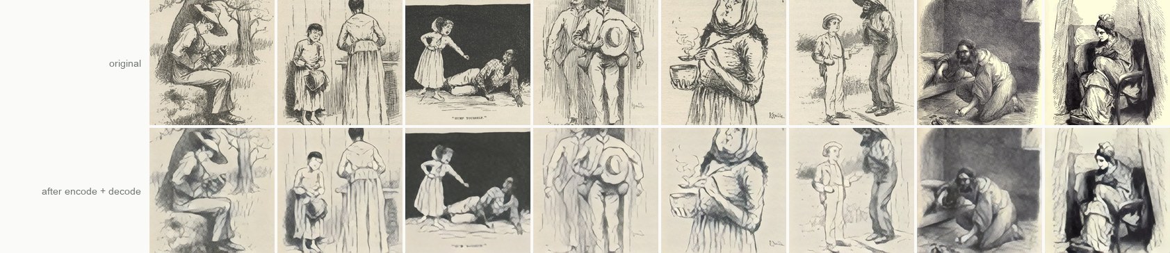
Eight validation images (top) and the same images after a round trip through the encoder and decoder (bottom). The composition and tone survive; fine hatching and small text do not. Whatever the diffusion model produces has to pass through this bottom row.
Compressing an image this much is lossy. The decoder gets back something close to the original, but never the original itself. Since the diffusion model only ever produces latents, and the decoder turns those latents into images, no image this system makes can be better than what the decoder is capable of reconstructing. Therefore, the autoencoder at this step sets a ceiling for the quality of the project.
To measure the ceiling, I took real images and ran them through the encoder and decoder. I scored the reconstructions against the originals using FID. A lower number here means two sets of images are more similar to each other. Two separate sets of real training images scored ~25.3 against each other, which is likely about as low as the number can go with this many samples. Real images after being passed through the autoencoder scored ~26.4. That number turned out to be useful, because it changed how I read all of the later results. When the diffusion model eventually reached a score of 46, it was 20 points from the best it could possibly do, given the autoencoder compression.
The first diffusion models I trained in latent space scored around 100, which was bad. The images looked washed out and blurry.
This was one of the places where working with an LLM to build out this model was most interesting. I didn't have a strong intuition about what had gone wrong, so I asked high-level questions, informed by some basic intuition about parts of the system I'd built so far. There were two parts of the system that I suspected could be at fault. Either the diffusion model was producing latents that were somehow off, or the decoder was taking slightly-off latents and turning them into badly-off images. My first guess was the decoder. It seemed plausible that it had only ever seen latents produced by its own encoder, and might break down on anything else.
Working with a frontier LLM through conversation helped by providing methods for testing this directly. The idea was to take latents from real images, which the decoder is known to handle well, deliberately corrupt them by adding a known amount of random noise, decode them, and score the result. If the decoder is fragile, a small amount of noise should produce a large jump in the score. If it isn't, the score should degrade gradually, and the size of the degradation would be useful information.
| latent noise added | FID after decoding |
|---|---|
| 0 | 26.3 |
| 0.1 | 26.9 |
| 0.2 | 30.3 |
| 0.35 | 43.9 |
| 0.5 | 70.6 |
The score degraded gradually, and so it seemed that the decoder was not fragile. Looking at the table, I could read the FID score as a measurement of error. A model scoring 100 was producing latents that were off by more than 0.5, which is a lot.
Learning that the issue likely wasn't in the compression step, the next guess was that the diffusion model likely hadn't trained long enough. The 10k steps that had been plenty for small 32-pixel images were probably insufficient for latents. So I resumed training. As was the case at several points of this project, the validation loss didn't move much over the course of many thousands of additional steps. Meanwhile, FID fell from 88 to 65. The model was getting visibly better, but the training objective showed nothing was changing.
Connecting text to images
So, now it's time to consider the bridge between text and image generation. The two halves I've described so far don't fit together in an obvious way. The text side reads text as input and produces vectors. The image side takes a noisy image and predicts how to remove the noise to produce an image.
The bridge is that the image model is given both a noisy image and text vectors as input. The image model is then trained so that its prediction of what to remove from the noise depends on both inputs. In practice, this means that at each layer, the image's patches may look at the caption's vectors and pull information from them, using the same attention mechanism the transformer uses, just pointed at the text instead of at other patches. Over the course of a few dozen denoising steps, a de-noised image emerges that is influenced by the caption. That is the whole mechanism!
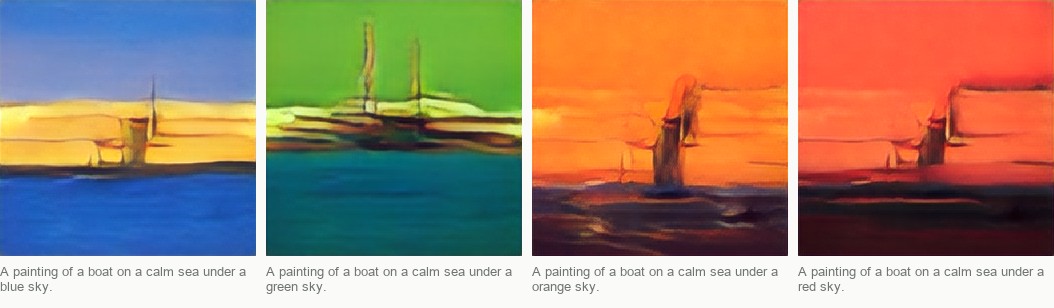
The same sentence with the word describing color changed, rendered four times from the same starting noise.
Up to this point, the image model had only been steered by a small discrete set of category labels, like "portrait" or "landscape." However, unlike a label, a descriptive caption is an arbitrary sentence represented as a sequence of tokens, to be embedded by the text side of the model, into vector representation.
My first approach was to use the transformer I'd already trained. When it reads text input, each layer produces a vector for each token, and those vectors are the model's "understanding" of the text so far. I fed them to the image model directly. I also tried a second approach, involving training a small version of CLIP myself.
CLIP, which I'll describe in a moment, learns to connect text and image pairs. The dataset I was working with had 78k paintings with captions, so I used the transformer as the text half and trained an image half alongside it. Both approaches worked, in that the image model learned to respond to captions. However, neither worked especially well.
Intuitively, it makes sense that these approaches wouldn't work well. Semantically, there is likely an enormous gap between the space of information encoded by the captioned images, and the space of information embedding the 20 novels used to train the transformer. The transformer could produce somewhat believable next-tokens, but at no point in training did I connect the token "boat" to what a boat looks like.
CLIP is a pair of models released by OpenAI in 2021 on about 400 million image-caption pairs from the internet. One model reads images, the other reads text. Each model produces a vector of length 512. The two were trained so that an image and a caption that belong together produce vectors that are close together in that 512-dimensional space. What makes this valuable for this project is that CLIP's text model has, in effect, already "learned" what pictures look like on a large dataset, containing a large number of different kinds of images and captions. When it encodes a caption, the numbers it produces are shaped by hundreds of millions of images.
So, in the end, the frozen CLIP encoder won, and my transformer did not make it into the final model. Though I learned something by building it, it did not provide the same depth of output as the pre-trained CLIP.
Connecting CLIP to the image model is relatively simple. CLIP transforms the caption into a short sequence of vectors, one per word or so. A small learned layer maps those vectors into the image model's own input size, and at each layer of the image model, the image tokens are allowed to look at the caption vectors and pull information from them. This is the same attention mechanism the transformer uses, just pointed at the text instead of at other image tokens. The pre-trained CLIP itself stays frozen throughout this process. The image model is then trained using input from CLIP.
One block of the image model with its two conditioning paths. The timestep modulates each normalization and gates each residual connection; the caption enters only through cross-attention, behind a projection that starts at zero.
The more difficult question was how to measure whether there was good, interpretable correlation between the images and the captions. I realized that looking at them each individually wouldn't scale well! I imagine that it's also easy to fool yourself when you want the images to look as if they correlate to the captions.
The approach I settled on is called retrieval. I generated an image for each of a set of held-out captions, then passed each image to another CLIP model, along with all of the captions, ranked them accordingly. When the judge model ranked the correct caption first, that counted as a hit. The ratio of hits was the score.
It's interesting to consider what the judge CLIP was measuring. A CLIP similarity score between an image and its caption is a number that mixes two different things together. It goes up when the image matches the caption, which is the objective. But, some images might score well against almost any caption. Some images in CLIP space sit close to lots of captions at once, while, on the other hand, a blurry or very distinctive image could be embedded far from all of them. So, an image can get a high score with its own caption because it's the kind of image the judge would rate highly in general. Using only this number, there's no way to why the image ranked the way it did.
To mitigate this, I added a control. For each image, I also scored it against the wrong captions, the ones belonging to other images, and reported the difference between the correct-caption score and the average incorrect-caption score. The incorrect-caption score captures how much the judge prefers the image, regardless of caption.
| judge | similarity to correct caption | to incorrect captions | margin |
|---|---|---|---|
| OpenAI B/32 | 0.2828 | 0.2054 | 0.0774 |
| LAION B/32 | 0.2794 | 0.1458 | 0.1336 |
The control makes the ranking flip. By raw score, the OpenAI judge looks better; by margin over wrong captions, the LAION judge is nearly twice as discriminating.
I ran two judges, two versions of CLIP trained on different data by two different orgs. One was trained by OpenAI, and the other by LAION, a non-profit that trained its own version on a large open dataset of image-caption pairs. Going by the raw score, the OpenAI judge gave the images a higher similarity to their captions, 0.283 against 0.279, so it seemed like the stronger judge. But it also gave them a much higher similarity to the incorrect captions, 0.205 against 0.146. Once that baseline was subtracted, the LAION judge's margin was approximately twice as large.
With these metrics, I could now measure whether a change to the model made the images follow their captions "better" or "worse" in some plausibly objective way. The first thing I measured was guidance, a setting that controls how strongly the caption's influence is applied to the final image. During training, the caption is left out some of the time, so the model learns to predict both with it and without it. At generation time, you take the difference between those two predictions and push the result further in the caption's direction. The guidance scale is the multiplier on that difference. At a scale of 1, you use the captioned prediction as is; at a scale of 5, you add the difference 5X over. In other words, whatever the caption changed about the prediction is exaggerated by that multiplier. A larger value here, and the images follow their captions more closely, but may start to look less natural.
I had set the scale to 2 initially, for the small class-label experiments. Going from 2 to 5 improved both the image quality score and the caption-adherence score. One of the nice things about guidance is that it's applied at generation time, so no re-training was necessary to experiment with different values.
| scale | FID | caption retrieval (R@1) | margin |
|---|---|---|---|
| 2 | 50.79 | 0.190 | 0.1336 |
| 5 | 46.49 | 0.321 | 0.1630 |
| 8 | 47.14 | 0.364 | 0.1674 |
The retrieval and margin columns above come from the LAION judge. Both judges in the earlier table are CLIP models with the same architecture.
In the end, these metrics are difficult to interpret, and the output is still subjective. Playing with the guidance and observing the outputs with the eye, it's often difficult to say what value produces "better" results, though the value does have a profound visual effect. I suspect this would become much more visually interesting and possibly interpretable for a diffusion model at much larger scale.
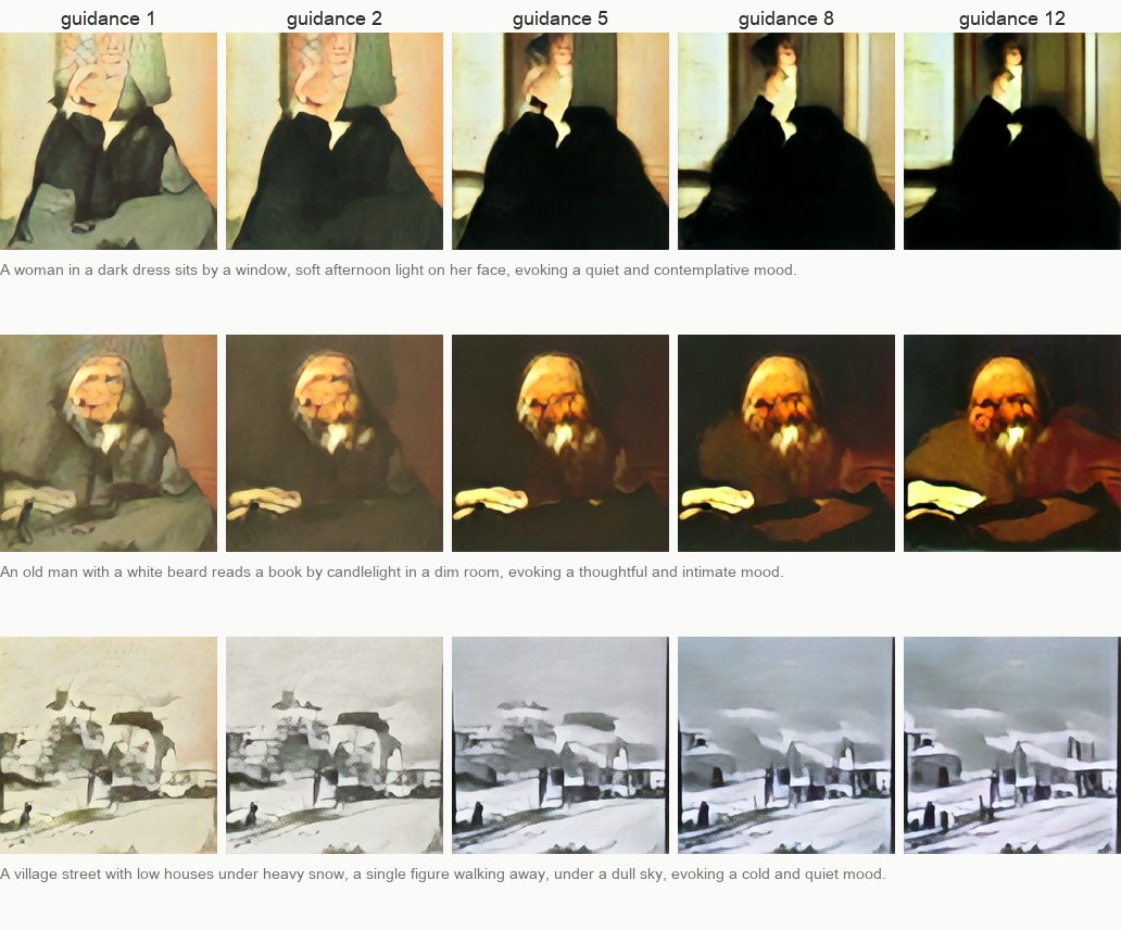
Three prompts at guidance 1, 2, 5, 8 and 12, each row starting from the same noise. At 1 the images are pale and loosely drawn; by 5 the subject and the lighting often more closely match the caption; by 12, the contrast and saturation are turned up dramatically.
Rendering books
With the model in a reasonably final state, I came back to the original idea and rendered some books, if only because they provide interesting descriptions of varied scenes. Paragraphs of text make poor prompts for this model. It trained on one-sentence captions, but CLIP's text encoder truncates anything past 77 tokens. So, I used the same local Qwen model that wrote the training captions to write a one-sentence scene summary of each paragraph, in the same register as those captions (a subject, a setting, the light, a mood), and used the summary as the prompt. I decided to set the starting noise to be the same within each chapter, so images generated from the same chapter would share a similar starting structure, and the differences between them are determined strictly by the text.
I've explored rendering a hundred paragraphs each from Heart of Darkness, Moby Dick, and To the Lighthouse. The whole run for a book takes about five minutes on my laptop; most of that time is spent by the local LLM writing summaries. The hundred frames themselves take under a minute. A few of the frames I found interesting are below.
(Note: the sentence shown below each image is the local Qwen model's summary of a paragraph of the novel, as mentioned; it is not the novel's text itself.
Moby Dick
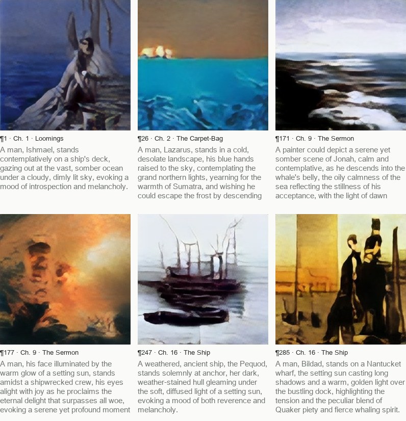
Six frames from the first sixteen chapters of Moby Dick. The text under each frame is the one-sentence summary of the paragraph written by the local Qwen model. Starting noise is shared within a chapter.
To the Lighthouse
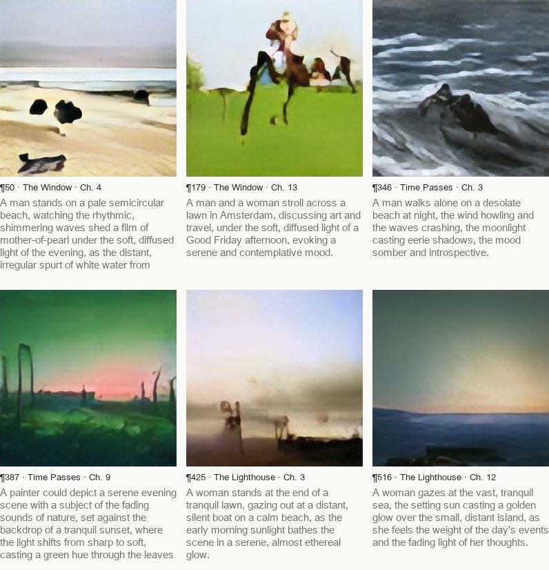
Six frames from To the Lighthouse, across all three parts of the novel. As above, the text under each frame is the local model's summary of the paragraph, used as the prompt.
A wide front end and a narrow back end
Stepping back from the individual experiments, I think the bottleneck in this project may be fairly straightforward. The front end, CLIP, is general. It was trained on ~400 million captions covering photographs, product shots, screenshots, and everything else on the internet, and it can describe nearly any sentence. The back end, the diffusion model, is very narrow in comparison. It has only ever seen 78,000 paintings (large enough to be interesting, but much smaller than the set of images used to train CLIP), described by a single locally-run captioning model. It only knows how to generate images in some small subset of CLIP's space. So, a caption like "a neon sign in the rain" or "a motorcycle on a winding road" is embedded by CLIP in a vector that represents that text in a well-structured and generally coherent space, and then lands on a part of the map the back end (the image model tasked with producing a corresponding image) has no representation for. I suspect the best it can do is fall back to loosely structured noise.
To make this concrete, I rendered two sets of eight sentences with the same seed and the same starting noise, so that the only difference between the two sets is the text. The first set is written in the style of the training captions and describes the kinds of subjects the paintings contain. The second set describes things CLIP has certainly seen among its 400 million captions, but the diffusion model has likely not seen.
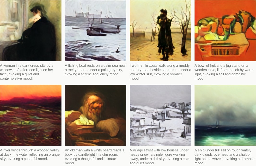
Eight prompts written in a similar style to the training captions. The model produces plausible paintings.
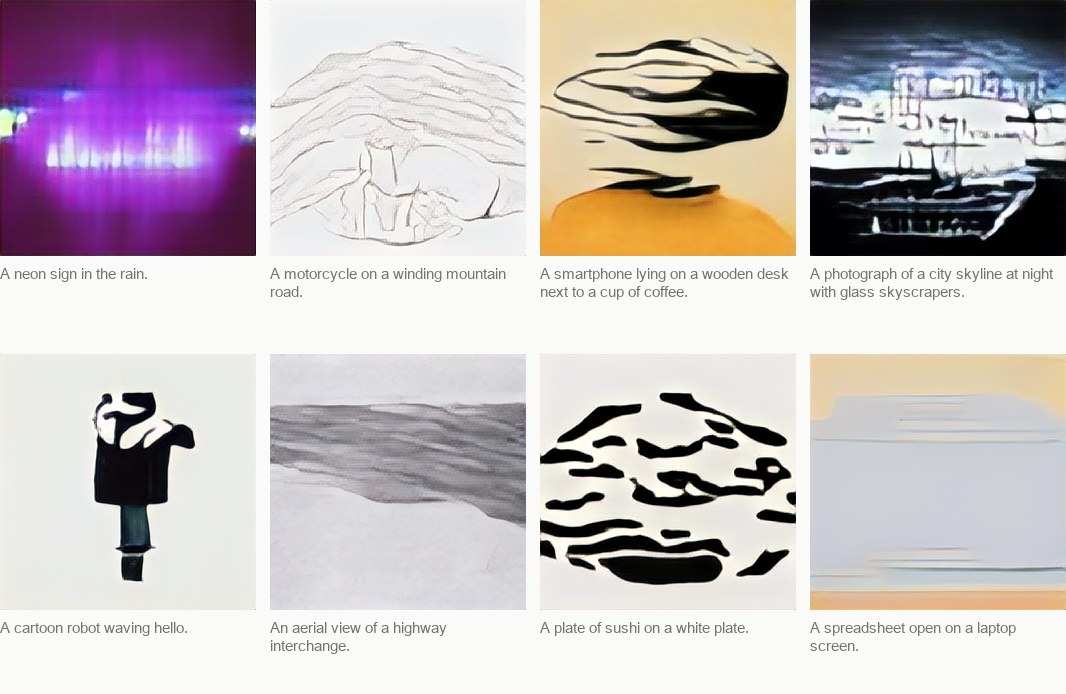
Eight prompts from outside the training distribution, same seed and noise.
I suspect the most direct approach for improving the model to produce "more realistic" output (though that wasn't my objective) is to expose the image model to much more data. Stable Diffusion (v1) also keeps a frozen CLIP text encoder in front, a larger one (ViT-L/14) than the ViT-B/32 used here. However, the bigger difference is in the back end, as its diffusion model was trained on LAION-2B-en, roughly two billion image-caption pairs, and then further on filtered subsets of it. Perhaps there are other options (I have a note to learn about unCLIP), but it seems intuitive that the ceiling on what the image model can generate is set by what it has seen during training.
The model as built
| quantity | value |
|---|---|
| total parameters | 40,718,608 |
| d_model / layers / heads | 384 / 12 / 6 |
| head dimension | 64 |
| patch size | 2 |
| latent grid | 32×32×4 → 16×16 = 256 tokens of 16 |
| objective | flow matching |
| text encoder | openai/clip-vit-base-patch32, frozen, causally masked |
| text interface | 8,257,536 params (20.3%) |
| conditioning | cross-attention; adaLN-Zero for timestep |
| autoencoder | 20,943,435 params; 8.56M encoder, 12.39M decoder |
| latent scale factor | 0.915 |
| training images | 78,308 |
| best checkpoint | step 64,500 of a 150,000-step budget |
| sampler for all reported figures | Heun, 25 steps (49 network evaluations) |
| best FID | 46.49 at guidance 5, N = 4,096 |
| autoencoder floor | 26.39 |
| real-versus-real floor | 25.26 |